by Daniel Schaffer and Phillip Compeau

Introduction

This is the first of a collection of assignments provided to students in Great Ideas in Computational Biology in which we will use data and software produced by others to draw conclusions about the SARS-CoV-2 virus that has caused the COVID-19 pandemic. In this sense, we are “research parasites”, a term coined by a now infamous 2016 editorial in the New England Journal of Medicine:

A … concern held by some is that a new class of research person will emerge — people who had nothing to do with the design and execution of the study but use another group’s data for their own ends, possibly stealing from the research productivity planned by the data gatherers, or even use the data to try to disprove what the original investigators had posited. There is concern among some front- line researchers that the system will be taken over by what some researchers have characterized as “research parasites.”

Just as we started this course with a discussion of how genomes are assembled, we start our study of SARS-CoV-2 by assembling its genome. This task was first completed on January 25, 2020 using a sample collected from the first known human patient .

Many patient DNA or RNA samples taken from swabs are metagenomic, meaning that they capture genetic material not only from the virus but also other viruses, bacteria, and even human cells. This means that researchers either have to apply an algorithm that is able to assemble genomes from information derived from multiple species, or they need to perform additional laboratory work to isolate the viral information. The researchers who assembled the first SARS-CoV-2 genome did the former, wrangling a 30,000 base pair genome out of a file consisting of 8 billion base pairs, most of which do not derive from SARS-CoV-2. If genome assembly is like assembling a puzzle, metagenome assembly is like assembling multiple similar puzzles from a jumbled set of pieces.

To prevent the complications of a metagenomics sample, we will work with a different viral read dataset that was sampled directly from an infected cultured cell.

Sequencing a virus is more straightforward than assembling a bacterium for a couple of reasons. First, the virus’s genome is much shorter. Second, SARS-CoV-2 is an RNA virus, meaning that its genome does not contain DNA, but rather a single (linear) strand of RNA, which is single-stranded; as a result, we do not encounter the complications that we do when assembling double-stranded DNA. Researchers convert RNA to DNA by using an enzyme called reverse transcriptase, a molecular tool that was invented by viruses to help them replicate their genome and now has been borrowed by humans to help us sequence this genome.

In this assignment, we will assemble the SARS-CoV-2 genome, and then we will annotate the contigs resulting from this assembly, meaning that we will compare our genome against a database of known genomes to label putative genes. Knowing the locations of these genes will allow us to study them in future work.

Getting started with Galaxy

To assemble the genome from the reads, we will be using the SPAdes assembler that is built upon a de Bruijn graph approach and is the most cited genome assembler of all time. To run SPAdes, we will use the Australian service of Galaxy, an open source project that allows us to run often testy bioinformatics software in the cloud without the hassle of dealing with local installations. Please follow these step-by-step instructions to register on Galaxy and run SPAdes:

First, create an account on Galaxy at https://usegalaxy.org.au/login. You don’t need to use your university email address, because we are only grading the results of your analysis. Your “public name” can be whatever you like, but you should fill out all fields. After creating an account, log in to Galaxy.

Click on the plus ‘+’ on the top right of the page and create a new “history” (i.e., project that will contain data and the results of software runs) named “SARS-CoV-2”. All of the following analysis will be performed under this history.

Grabbing some sequencing data

The National Center for Biotechnology Information (NCBI) hosts an enormous amount of publicly available biological data. You may be interested in their website for SARS-CoV-2 (https://www.ncbi.nlm.nih.gov/sars-cov-2/), which contains sequencing data from hundreds of thousands of sequencing “runs”. These runs are stored in an arm of NCBI called the Sequence Read Archive (SRA), where researchers can upload sequencing reads from their experiments.

Our dataset of interest has the SRA identifier SRR11528307, and its homepage can be found here: https://trace.ncbi.nlm.nih.gov/Traces/sra/?run=SRR11528307. We can see at this page that the dataset contains approximately 719,800 reads (“spots”), that the technology is “Illumina”, and that the layout is “paired”. These are short paired-end reads produced by Illumina’s popular sequencing by synthesis approach that we learned about.

Exercise 1: How many nucleotide bases are found in this file? What is the GC-content of the reads? (That is, the percentage of reads that are either G or C.)

The coverage of a collection of sequencing reads is defined as the number of nucleotides in the reads, divided by the length of the genome from which they derive. It tells us, on average, the number of sequencing reads in which each nucleotide from the genome appears.

Exercise 2: We know that the original SARS-CoV genome from the 2003 outbreak has approximately 30,000 nucleotides. If the SARS-CoV-2 genome has length 30,000 nucleotides, then what is the coverage of this read dataset?

Clicking on the “Reads” tab will allow us to see ten read-pairs at a time. Each read is in FASTA format, meaning that the read has a header beginning with the “>” symbol identifying the read, followed by the read itself.

Exercise 3: What is the read-pair at spot #15213? Why do you think that one read is shorter than the other?

Now that we know where our data is contained, let’s import it into Galaxy. To do so, go back to Galaxy and on the left side of the page, under "Get Data“, click “Download and Extract Reads in FASTQ format from NCBI SRA”. Make sure that “select input type” shows “SRR accession”, and type our accession ID (SRR11528307) into the field below. You may want to click “Yes” for “Email notification”, although the job should not take more than five minutes to run. Then click “Run Tool”. You should see the job added to your history on the right; it will turn green when it is finished.

FASTQ format and Phred quality scores

When the job turns green, click on “Paired-end data (fast-dump)” under your history on the right side of the page, then click on "SRR11528307", and then click on the “eye” symbol next to "forward". It may take a few seconds to load the file.

This file is in FASTQ format, an extension of FASTA format in which each read is represented over four lines described as follows.

1. A header beginning with the “@” symbol and labeling the read. Notice that because these are read pairs, the first two reads’ headers are the same and end with “/1” and “/2”.
2. The read as a sequence of nucleotides.
3. A line containing a “+” symbol to indicate the end of nucleotides. This line may havemore header information, but doesn’t for this dataset.
4. A collection of ASCII symbols representing Phred quality scores, described below. The i-th quality score corresponds to the i-th nucleotide in the read.

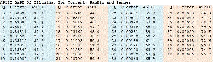
A given base returned as the result of a sequencing run is assigned a quality score Q based on an estimate of how likely this base is correct. Because many bases are very reliable, this computation is done on a logarithmic scale. In particular, once we compute the probability p that a base is incorrect, we set Q = -10 log₁₀(p) and assign the base the ASCII symbol corresponding to Q + 33. For example, if p is 0.001, then log₁₀(p) is -3, and so Q is equal to 30, and we assign this base the ASCII symbol corresponding to 30 + 33, which is “?”. As a result, the lower the value of p, the higher the quality score Q. The Phred quality score table is shown in the figure below.

Phred scores are helpful for a variety of reasons. For example, researchers will throw out reads having a significant number of bases that do not meet a certain Phred score threshold, especially if the reads have high coverage.

Exercise 4: How would Phred scores be useful when applying the de Bruijn graph approach to genome assembly?

Exercise 5: In class, we learned about the sequencing by synthesis approached used by Illumina for sequencing reads. What do you think that Illumina considers to determine the quality score of a given base?

Exercise 6: Head back to the SRA page for our dataset. In the “Metadata” tab, there is small text that says “Quality graph”. You may need to click “bigger” to see this graph, which is a histogram of Phred quality scores over the entire dataset. Interpret this chart. Are the quality scores good? What makes you think so?

Exercise 7: Return to Galaxy to viewing the forward component of your SRR11528307 dataset. Use CTRL + F or COMMAND + F to find the read with label “8595/1”? What are its quality scores? Are these quality scores good? Are there any nucleotides you are worried about? What might we do?

Assembling the SARS-CoV-2 genome

Now that we understand our data a bit better, we are ready to assemble the SARS-CoV-2 genome from our read set using SPAdes. Under Genomics Analysis → Assembly on the left side of the page, you will see over a dozen different assemblers. Click on SPAdes, which will take you to its homepage.

We will go through each of the settings offered and briefly explain them as well as what we are going to choose.

• Operation Mode: Set to “Assembly and error correction“. We want SPAdes to try and “error correct” reads, meaning that it looks for potentially troubling bases and correcting reads. For example, if a read matches another read exactly except for a single base with a very low quality score, we may want to error correct this read before we build a de Bruijn graph.
• Single-end or paired-end short-reads: Set to "Pair-end: list of dataset pairs“. Remember that we know these are paired-end reads.
  • FASTA/FASTQ file(s): collection: Set to "Pair-end data (fastq-dump)". (There should be only one option).
  • Type of paired reads: set to default (--pe), since we have paired-end reads.
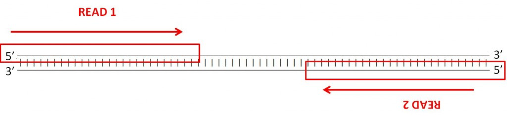
  • Select orientation of reads: Set to “FR(-><-)”. Remember that the convention is to always read DNA in the 5’ to 3’ direction. In forward-reverse read pairs, the first read is taken from one strand, and its pair is taken from the opposing strand, as the figure below illustrates.
  • Use an additional set of short-reads: this should be set to disabled, as we do not have another read dataset that we are incorporating. Algorithms sometimes can use multiple read datasets in order to improve the final assembly quality.

• Pipeline options: keep these unselected, as they provide additional functions that we will not need. If you’re interested, here is what they mean.
  • Careful: Select. The BWA tool is based on a Burrows-Wheeler transform approach to read mapping that we learn about later in the course.
  • Single cell mode: DO NOT select. This setting is used for bacterial projects when we have a bacterium that we cannot culture, and we only have DNA captured from a single cell.
  • Iontorrent: DO NOT select as these are Illumina reads. Iontorrent reads are produced by a different company (Oxford Nanopore) and are longer and typically less accurate.
  • Isolate: DO NOT select. If we had a high-coverage collection of reads of varying lengths, we might choose only the longest reads above some threshold (assuming they have sufficient quality) to save us some time in running the assembler. We are assembling a virus, so we don’t need a coverage cutoff.
• Select k-mer detection option: Set to “Auto”. SPAdes works by building de Bruijn graphs for several values of k. The default values are k = 21, 33, and 55. We have no a priori information that would lead us to change SPAdes’ default behavior, so we will let its “machine learning” choose the best values to use.
• Output final assembly graph (contigs)? Set to “Yes”
• Select optional output file(s): Keep all parameters ("Assembly graph", "Contigs", "Assembly graph with scaffolds", and "Scaffolds") selected. Because we want to see the contigs produced by SPAdes, and we would love to view the final assembly graph, which needs scaffolds.
• Email notification: We suggest setting to “Yes” so that you can leave this running andget notified when it’s done.

Keep all other parameters in their default setting. Here is a screen shot of the parameter settings we are using:

You are now ready to go! Click “Run Tool”. SPAdes should take 15-20 minutes to finish.

Analyzing the results of our assembly

Now that SPAdes has completed, we will analyze the results. As the previous exercise indicates, our work appears to have been quite successful.

Exercise 8: Click on the eye symbol (“view data”) next to the “contigs (fasta)” line on the right side. How many contigs did our assembly produce? (You will need to scroll down in order to see them.) What are their lengths? What do you think “coverage” means in this context?

SPAdes produced not only contigs but scaffolds, which are produced often by using additional information about the genome, which may involve comparison against related genomes. (In this case, the contigs and scaffolds are the same.)

We also produced an “assembly graph” as the result of our work, which is a version of the de Bruijn graph (after some cleaning steps involving bubble removal) in which maximal nonbranching paths have been compressed down and assigned to nodes, and if contigs x and y are known to overlap, we connect x to y with a directed edge. If you “view data” for the assembly graph by clicking the eye symbol next to "Assembly graph with scaffolds", then you will see that this graph has four nodes (in our run these nodes are labeled “8685”, “8687”, “8693”, and “8751”; furthermore, you will see that the strings labeling them have different lengths.

Next, scroll down to the bottom of the file. You will see the following lines (or something similar), which indicate the edge relationships in the graph.

L	8751	-	8685	-	77M
L	8751	-	8687	-	77M
L	8693	-	8685	+	77M
L	8693	-	8687	+	77M
P	NODE_1_length_29600_cov_2807.677743_1	8693-,8685+,8751+	*
P	NODE_2_length_147_cov_27.500000_1	8687+	*

The first four lines tell us the edge relationships (the "L" at the start of each line stands for “link”). For example, we see that node 8751 is connected to (overlaps with) node 8685. We also have additional information, which is that the node overlaps with the reverse complement of node 8685, so that we have inferred contigs that lie on opposing strands.

The bottom two lines tell us what the algorithm has inferred from the network as contigs. To do so, it consults read pairs where one member of the pair exists on one contig, and the other member of the pair is found on another contig, allowing it to conclude that these contigs must be adjacent.

In particular, the algorithm has formed contigs by overlapping reads “8693”, “8685”, and “8751” into contig 1, and leaving “8687” as a singleton that forms contig 2.

Now let’s visualize this assembly graph! To do so, we use a program called Bandage. Under “Assembly” on the left side of the page, click on “Bandage Image”. Under “Graphical Fragment Assembly” select "Assembly Graph with Scaffolds". Feel free to keep all other parameters the same (possibly opting for an email notification), and click “Run Tool”. The program should only take a couple of seconds to run.

Exercise 9: First, draw what you think that the graph will look like according to the edge information provided in the first four lines of the output shown above. Then, click the “eye” symbol to view the graph next to the image produced in the sidebar, and examine the image produced of the assembly graph. Do they match? Do you see the paths that were formed into contigs?

Aligning the two viruses

Because we have a single long contig, and the virus genomes are ultimately short, let’s align it against the original SARS-CoV genome from the 2003 outbreak to see how the two coronavirus genomes differ.

Exercise 10: We will align the two genomes as DNA strings rather than translating them to protein strings. Why do you think this is?

To align the SARS-CoV-2 genome against the original SARS-CoV genome, we will use the (affine) global alignment algorithm that we learned about in class, provided at NCBI at https://bit.ly/2NtCsWX under the accession ID NC_004718.3. To import this genome, we will use the “NCBI Accession Download” tool under “Get Data” on the left side of the Galaxy page. After clicking on this tool, follow these steps.

• Under “Select source for IDs”, select “Direct Entry”.
• Under ID List, type NC_004718.3.
• Keep the other parameters the same, add an Email notification if you like, and click “Run Tool”.

The tool should be very quick.

Now we are ready to align the two genomes. Under the “EMBOSS” section on the left side of the page, click “needle”, which is short for “Needleman-Wunsch global alignment”, the algorithm we learned about in class.

For sequence 1, select the contigs that we produced as the result of SPAdes. For sequence 2, select NC_004718.3. Keep the other parameters default (you may like to play around with these parameters later to see how they affect the outcome). After opting for an Email notification, click “Run Tool”. The algorithm should take a few minutes to run.

When the algorithm has finished, view its data. This will show the alignment, in which matches are shown with “|” symbols, mismatches are shown with “.” symbols, and indels do not have a symbol between the two rows.

Exercise 11: How many matched symbols does the alignment report? How many gap symbols?

Exercise 12: What do you notice about the ends of the alignment? What do you think happened when the genome was assembled?

Exercise 13: Scroll through the interior of the alignment. Do you notice any regions that appear to be more variable than other regions?=

Annotating the SARS-CoV-2 genome

Finally, we will annotate the SARS-CoV-2 genome, meaning that we will identify putative genes and then compare these genes against a database of known genes to find which ones align the best.

The identification of putative genes can be done in a variety of ways. One way to find these regions requires the observation that regions of DNA that are translated into protein start with a start codon (ATG) and end with a stop codon (TAG, TAA, or TGA). If a genome were random, then after encountering a start codon, we would expect to see a stop codon after about 64/3 ~ 21 codons. But real genes are typically much, much longer than 21 codons. As a result, in simple organisms like viruses and bacteria, a great way to find genes is to look for long stretches of codons connecting a start codon to a stop codon, with no intermediate stop codons.

Once we have found putative genes along the genome, we can compare them against a database of genes using an algorithm called BLAST that we will learn about soon.

These two steps are taken by our next tool, called Prokka, which is used to annotate the genomes of viruses, bacteria, and archaea. It can be found under “Annotation” on Galaxy. Under “Contigs to annotate”, select our contigs from the SPAdes run. Set “Kingdom” to “Viruses” and leave all other parameters to default. Note that our shorter contig will not be included in the annotation because Prokka only annotates contigs of length at least 200. Select whether you would like an Email on completion, and click “Run Tool”.

The entire process of annotating our genome should not take more than a few seconds. Isn’t bioinformatics great?

Prokka produces a collection of output files, which you might like to view. The .fna file contains the lone contig that survived. The .gff file contains regions identified by Prokka as genes. The .ffn file contains nucleotide sequences of the annotated genes, and the .faa file contains their translated amino acid sequences.

Exercise 14: First, view the .gff file containing regions identified by Prokka as putative genes. How many are there? What is the longest and shortest one?

Prokka contains the annotation information in these files, but what a biologist would really like is a visualization of its genes and what they have been predicted to be. So to visualize our annotation contained in the .gff file, we will use a genome browser tool called “JBrowse” that is found in the “Graph/Display” section on the left side of the page.

When running JBrowse, take the following steps.

• Reference genome to display. Select “Use a genome from history” and choose the .fna file.
• Click “Insert Track Group”.
• Click “Insert Annotation Track”.
• Select your .gff file from the Prokka output.
• Under “Email notification”, choose “Yes” if you like.
• Then click “Run Tool”.

JBrowse should be very quick. When it is finished, click view file, which is an HTML file that we can view in the browser. (It may take a moment to load.)

It seems like nothing is there, but on the left side of the page, click on “Prokka on data XXX: gff” to show our beautiful annotation of the SARS-CoV-2 genome. Zoom out to see it in all its glory. All the arrows point in the same direction to indicate that the genes are all found on the same strand of the genome. This makes sense because SARS-CoV-2 is an RNA virus, meaning that its genome has only one strand. (It would have been a very bad sign if some genes pointed in the opposite direction.)

You can click on the genes as you like to obtain information about their length and what in the database they were found to be similar to (if anything). For example, if you click on the first protein (Replicase polyprotein 1a), you will find that it was found to be similar to the protein with Uniprot ID (https://www.uniprot.org/uniprot/P0C6U8), which is the same gene in SARS-CoV. Note that the annotation score of this protein is high because there is so much experimental evidence backing up this protein. This means that if we find a putative gene that is a hit against it, we can have a high degree of certainty that our gene serves a similar function.

Exercise 15: Why do you think that two of the genes are labeled “hypothetical proteins”?

It may amaze you that such a tiny thing can wreak so much havoc. But now that we know this annotation, we can start investigating the virus’s individual genes. Which one should we focus on? How has the gene mutated as the virus spread around the world? And how do these mutations affect the function of the protein? We save these topics for the subject of future study.