
Phillip Compeau, Ph.D.
Teaching Professor
Asst Dean for Innovation in Computing Education
Computational Biology Department
Carnegie Mellon University
SARS-CoV-2 Spike Protein Structure Analysis Assignment
by Chris Lee and Phillip Compeau
Note: This challenge is adapted from a longer module that is part of my Biological Modeling project. If you enjoy this material, check out that course and its accompanying textbook at https://biologicalmodeling.org.
Introduction
In previous assignments, we assembled and annotated the SARS-CoV-2 genome, and we then examined how this genome is changing as the virus mutates within the human population. We saw that some regions of the genome are more variable than others compared to the SARS-CoV genome; we will focus on one of these regions, the gene encoding the spike protein.
In this assignment, we will place ourselves in the shoes of early SARS-CoV-2 researchers studying the new virus in January 2020 after the virus’s genome was published. We now ask ourselves two questions. First, can we use the virus’s genome to determine the structure of its spike protein? Second, once we know the structure of the SARS-CoV-2 spike protein, how does its structure and function differ from the same protein in SARS-CoV?
However, first we take a small detour to explain what we mean by the “structure” of a protein.
The four levels of protein structure
Protein structure is a broad term that encapsulates four different levels of description. A protein’s primary structure refers to the amino acid sequence of the polypeptide chain. The primary structure of human hemoglobin subunit alpha can be downloaded here, and the primary structure of the SARS-CoV-2 spike protein can be downloaded here.
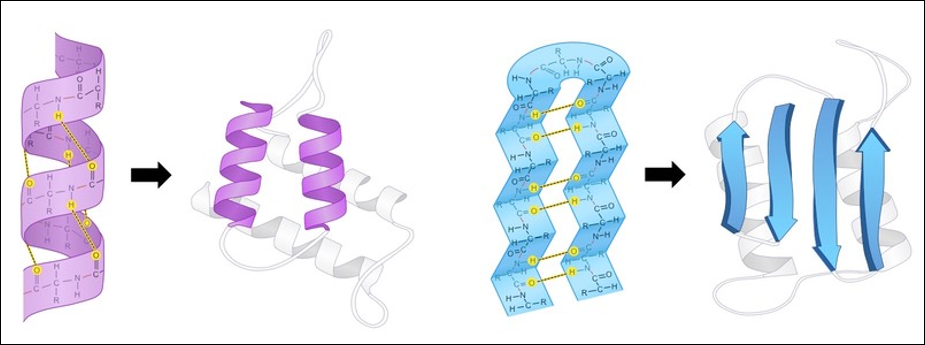
A protein’s secondary structure describes its highly regular, repeating intermediate substructures that form before the overall protein folding process completes. The two most common such substructures, shown in the figure below, are alpha helices and beta sheets. Alpha helices occur when nearby amino acids wrap around to form a tube structure; beta sheets occur when nearby amino acids line up side-by-side.
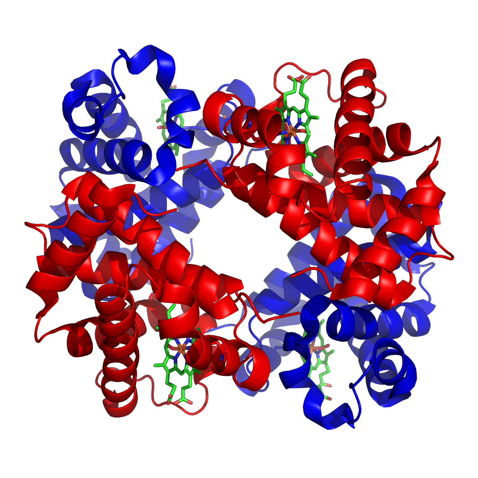
A protein’s tertiary structure describes its final 3D shape after the polypeptide chain has folded and is stable. Throughout this challenge, when discussing the “shape” or “structure” of a protein, we are almost exclusively referring to its tertiary structure. The figure below shows the tertiary structure of human hemoglobin subunit alpha. For the sake of simplicity, this figure does not show the position of every atom in the protein but rather represents the protein shape as a composition of secondary structures.

Finally, some proteins have a quaternary structure, which describes the protein’s interaction with other copies of itself to form a single functional unit, or a multimer. Many proteins do not have a quaternary structure and function as an independent monomer. The figure below shows the quaternary structure of hemoglobin, which is a multimer consisting of two alpha subunits and two beta subunits.
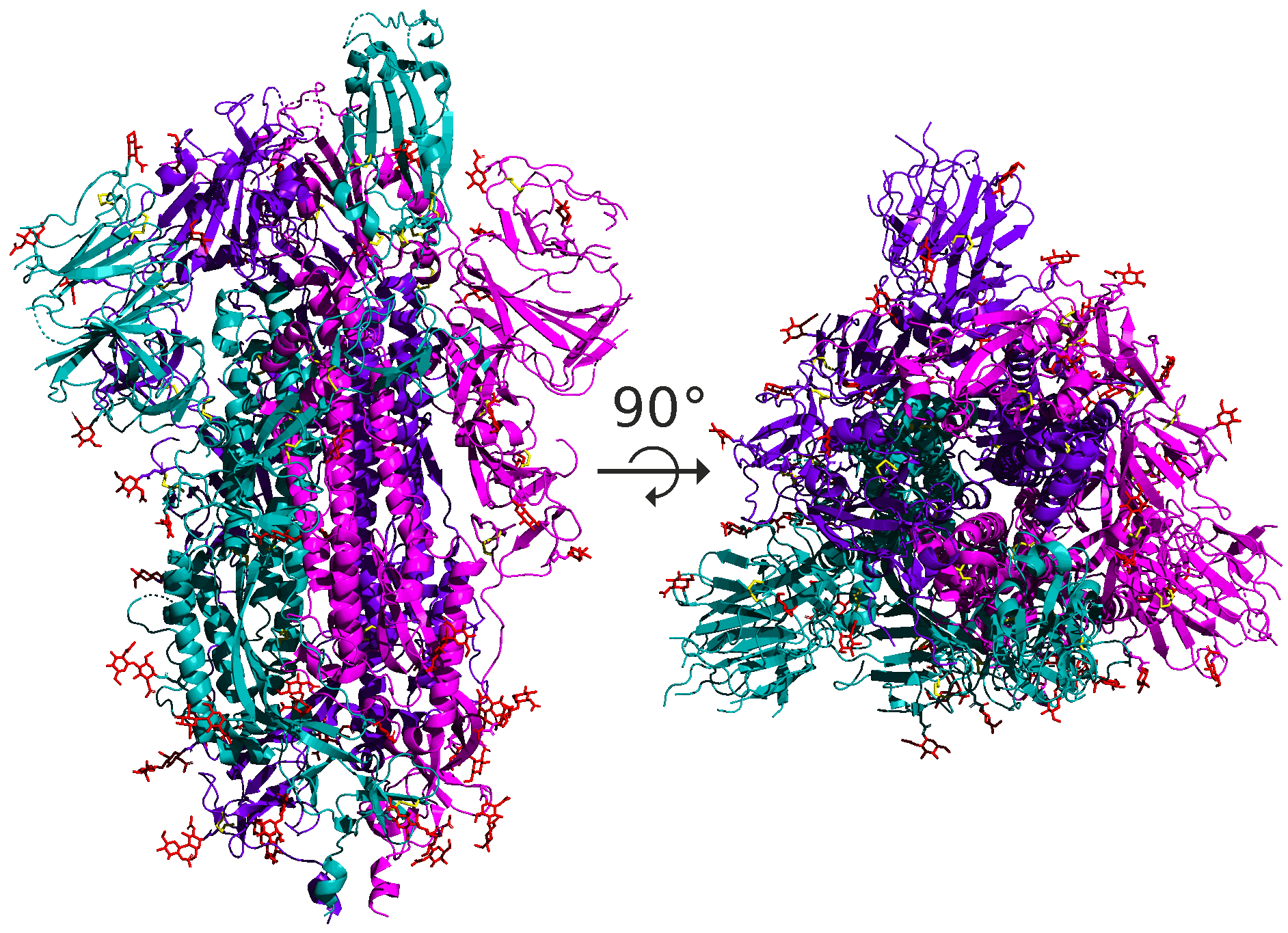
As for SARS-CoV and SARS-CoV-2, the spike protein is a homotrimer, meaning that it is formed of three essentially identical units called chains, each one translated from the corresponding region of the coronavirus’s genome; these chains are colored differently in the figure below. When discussing the structure of the spike protein, we typically are referring to the structure of a single chain.
The structural units making up proteins are often hierarchical, and the spike protein is no exception. Each spike protein chain is a dimer, consisting of two subunits called S1 and S2. Each of these subunits further divides into protein domains, distinct structural units within the protein that fold independently and are typically responsible for a specific interaction or function. For example, the SARS-CoV-2 spike protein has a receptor binding domain (RBD) located on the S1 subunit of the spike protein that is responsible for interacting with the human ACE2 enzyme; the rest of the protein does not come into contact with ACE2. We will say more about the RBD soon.
Proteins seek the lowest energy conformation
Now that we know a bit more about how protein structure is defined, we will discuss why proteins fold in the same way every time. In other words, what are the factors driving the magic algorithm?
Amino acids’ side chain variety causes amino acids to have different chemical properties, which can lead to different conformations being more chemically “preferable” than others. For example, the table below groups the twenty amino acids commonly occurring in proteins according to chemical properties. Nine of these amino acids are hydrophobic (also called nonpolar), meaning that their side chains tend to be repelled by water, and so we tend to find these amino acids sheltered from the environment on the interior of the protein.
We can therefore view protein folding as finding the tertiary structure that is the most stable given a polypeptide’s primary structure. Any system of chemical reactions tends to move toward equilibrium, and the same principle is true of protein folding; when a protein folds into its final structure, it is obtaining a conformation that is as chemically stable as possible.
To be more precise, the potential energy (sometimes called free energy) of a molecule is the energy stored within an object due to its position, state, and arrangement. In molecular mechanics, the potential energy is made up of the sum of bonded energy and non-bonded energy.
As the protein bends and twists into a stable conformation, bonded energy derives from the protein’s covalent bonds, as well as the bond angles within and between adjacent amino acids.
Non-bonded energy comprises electrostatic interactions and van der Waals interactions. Electrostatic interactions refer to the attraction and repulsion force from the electric charge between pairs of charged amino acids. Two of the twenty standard amino acids (arginine and lysine) are positively charged, and two (aspartic acid and glutamic acid) are negatively charged. Two nearby amino acids of opposite charge may interact to form a salt bridge. Conformations that contain salt bridges and keep apart similarly charged amino acids will therefore have lower free energy contributed by electrostatic interactions.
As for van der Waals interactions, atoms are dynamic systems, with electrons constantly buzzing around the nucleus, as shown in the figure below.
However, due to random chance, the electrons in an atom could momentarily be unevenly distributed on one side of the nucleus. Because electrons are negatively charged, this uneven distribution will cause the atom to have a temporary negative charge on the side with the excess electrons and a temporary positive charge on the opposite side. As a result of this charge, one side of the atom may attract only the oppositely charged components of another atom, creating an induced dipole in that atom in turn as shown in the figure below. Van der Waals forces refer to the attraction and repulsion between atoms because of induced dipoles.
As the protein folds, it seeks a conformation of lowest total potential energy based on the combination of all these forces. For an analogy, imagine a ball on a slope, as shown in the following figure. The ball will tend to move down the slope unless it is pushed uphill by some outside force, making it unlikely that the ball will wind up at the top of a hill. We will keep this analogy in mind as we return to the problem of protein structure prediction.
Structure prediction with homology modeling
In a priori structure prediction, we attempt to reconstruct the (tertiary) structure of a protein directly from its amino acid sequence, without taking any known structures into account. Unfortunately, the algorithms implementing a priori structure prediction take a very long time to run; in fact, some publicly available a priori structure prediction software caps the length of the protein.
Since the SARS-CoV-2 spike protein gene encodes a polypeptide chain with 1281 amino acids, we will instead turn our attention to homology modeling, in which we use a database of experimentally validated structures to increase the accuracy and efficiency of structure prediction.
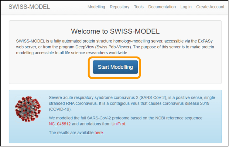
There are several publicly available resources for homology modeling; we will use a web server called SWISS-MODEL. To run SWISS-MODEL, first download the sequence of the spike protein chain: SARS-CoV-2 spike protein chain. Next, go to the main SWISS-MODEL website and click Start Modelling.
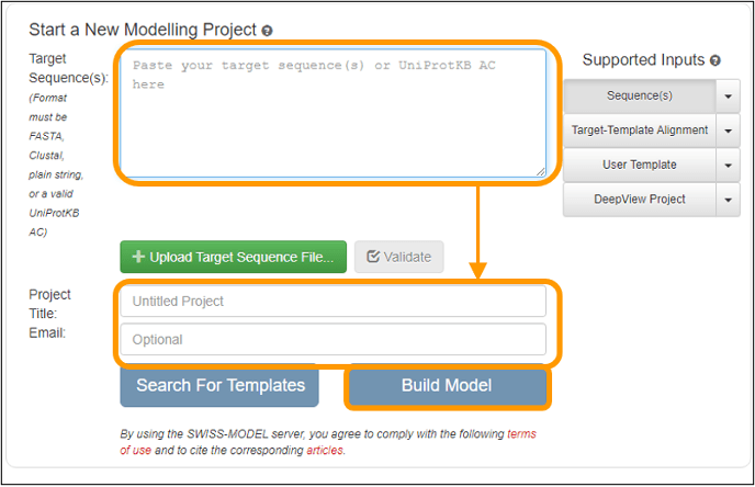
On the next page, copy and paste the sequence into the Target Sequence(s): box. Name your project and enter an email address to get a notification of when your results are ready. Finally, click Build Model to submit the job request. Note that you do not need to specify that you want to use the SARS-CoV spike protein as a template because the software will automatically search for a template for you (and find this template).
Important note: your results may take between an hour and a day to finish depending on how busy the server is. When you receive an email notification, follow the link provided and you can download the final models produced.
When SWISS-MODEL finishes, visit the results page. You will see a collection of structure models produced as a result of the modeling process. By default, an image of the “model 1” predicted protein is shown on the right of the page. Feel free to explore this model by clicking to rotate it.
Exercise 1: SWISS-MODEL returned multiple results. Give two reasons why returning multiple results would be helpful for researchers.
Exercise 2: For each of the models produced by SWISS-MODEL, explain what template was used, which organism it came from, and what its sequence identity is with the SARS-CoV-2 molecule.
SWISS-MODEL provides metrics to attempt to determine the quality of each of the models that it predicts. We will allow you to explore these metrics at the SWISS-MODEL documentation but will mention that one of the metrics is QMEAN, which attempts to quantify how well a modeled structure compares against what we would “expect” to see in experimental structures. SWISS-MODEL furthermore colors the predicted structure on a spectrum based on QMEAN quality scores, with blue regions representing high similarity, and red regions representing lower similarity. By clicking on the image of different models on the left, you can see how the models differ.
In the meantime, we want to save the models that we produced so that they can be used in other analyses. To do so, click the download icon near the top of the page and save the models to your computer.
Comparing a predicted spike protein structure against SARS-CoV-2
Our prediction of the SARS-CoV-2 spike protein mimics the work of many researchers in January 2020, which included the contributions of volunteers’ computers from around the world.
Meanwhile, other scientists were working on verifying the structure of the protein experimentally. On February 25, 2020, researchers from the Seattle Structural Genomics Center for Infectious Disease deposited the result of a cryo-EM experiment determining the structure of the spike protein to the Protein Data Bank (PDB) as entry 6vxx. Cryo-EM is described in the following YouTube video if you are interested.
Our goal is to compare the models that SWISS-MODEL predicted against the validated structure of SARS-CoV-2. To do so, we will need to have a file format that represents the tertiary structure of a protein. We will use .pdb format, which is illustrated in the figure below. Each atom in the protein is labeled according to several different pieces of information, including:
- the element from which the atom derives;
- the amino acid in which the atom is contained;
- the chain on which this amino acid is found;
- the position of the amino acid within this chain; and
- the 3D coordinates (x, y, z) of the atom in angstroms (10-10 meters).
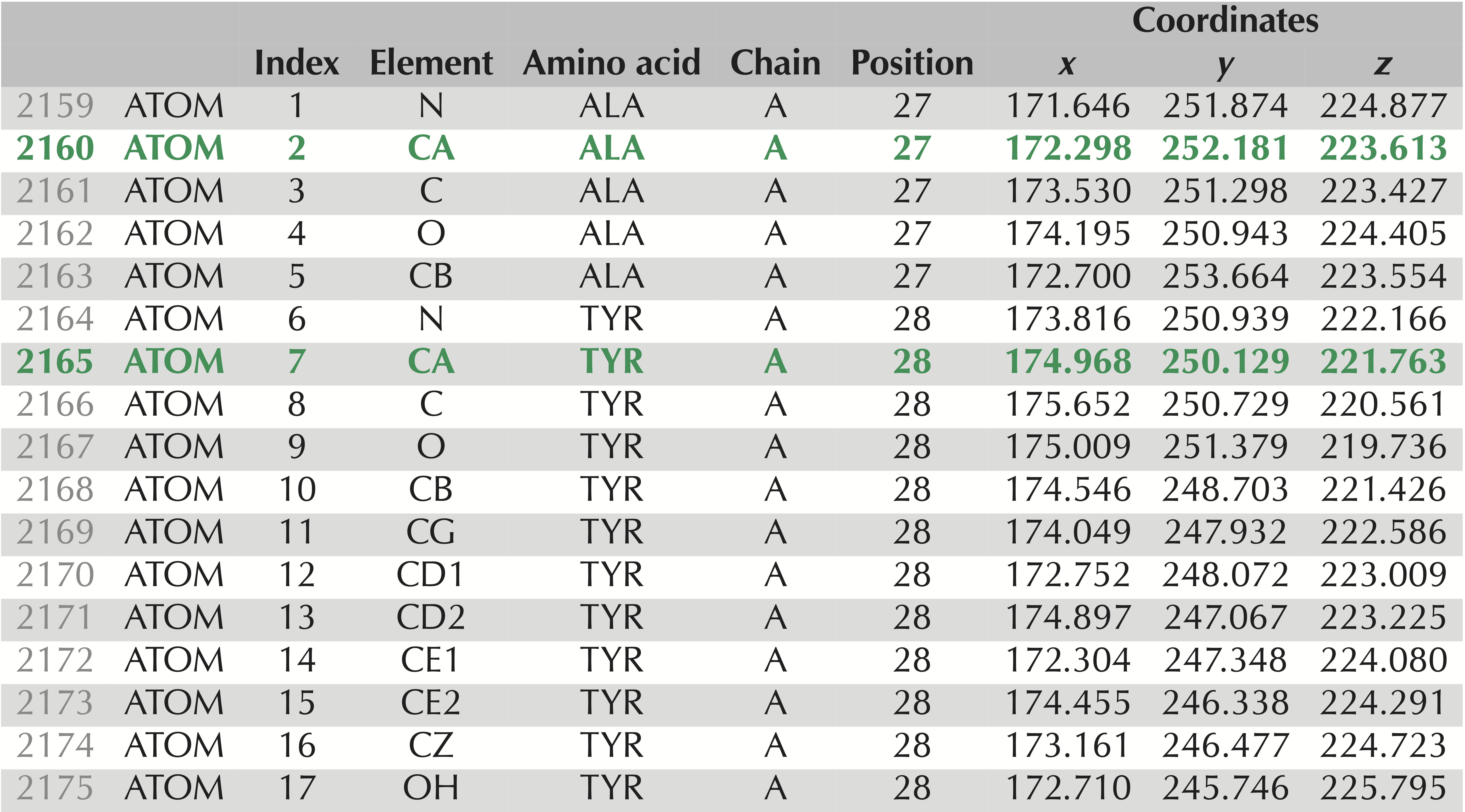
.pdb file for the experimentally verified SARS-CoV-2 spike protein structure, PDB entry 6vxx. These 17 lines contain information on the atoms taken from two amino acids, alanine and tyrosine. The rows corresponding to these amino acids’ alpha carbons are shown in green and appear as “CA” under the “Element” column. We have labeled the columns to make it clear what each column corresponds to: “Index” refers to the number of the amino acid; “Element” identifies the chemical element to which this atom corresponds; “Chain” indicates which chain the atom is found on; “Position” identifies the position in the protein of the amino acid from which the atom is taken; “Coordinates” indicates the x, y, and z coordinates of the atom’s location (in angstroms).Open the folder that you downloaded from SWISS-MODEL. You will see a directory corresponding to each of the models that the software predicted. Within each directory, there is a model.pdb file that can be opened with a text editor.
Exercise 3: Provide the first ten lines corresponding to atomic positions of your model 1. (Note: answers may vary here.)
We now would like to compare the known SARS-CoV-2 protein structure against a structure predicted by a model, which is an example of the more general problem of comparing two shapes.
Comparing two shapes with the Kabsch algorithm
Consider the two shapes in the figure below. How similar are they?
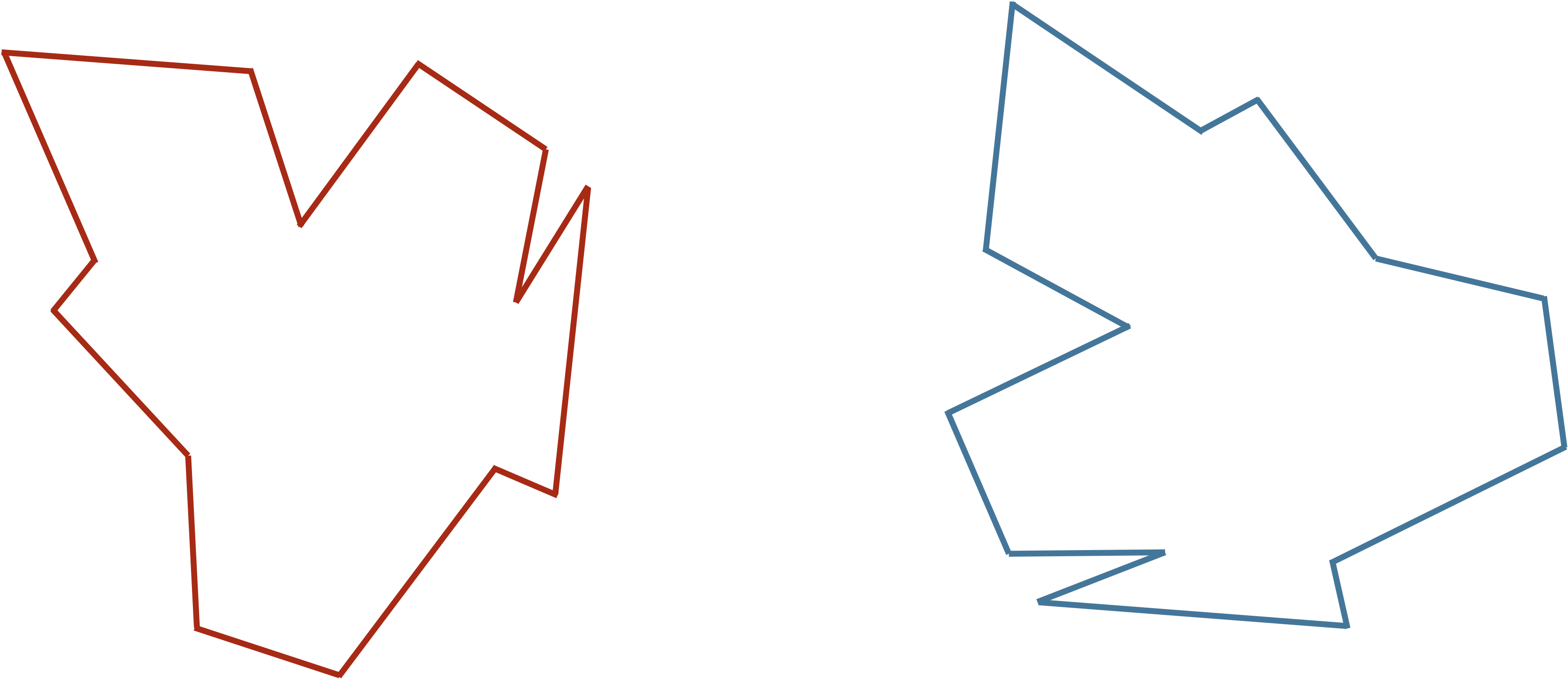
If you think you have a good handle on comparing the above two shapes, then it is because humans have very highly evolved eyes and brains. But training a computer to detect and differentiate objects is more difficult than you think!
We would like to develop a distance function d(S, T) quantifying how different two shapes S and T are. If S and T are the same, then d(S, T) should be equal to zero; the more different S and T become, the larger d should become.
You may have noticed that the two shapes in the preceding figure are, in fact, identical. To demonstrate that this is true, we can first move the red shape to superimpose it over the blue shape, then flip the red shape, and finally rotate it so that its boundary coincides with the blue shape, as shown in the animation below. In general, if a shape S can be translated, flipped, and/or rotated to produce shape T, then S and T are the same shape, and so d(S, T) should be equal to zero. The question is what d(S, T) should be if S and T are not the same shape.
Our idea for defining d(S, T), then, is first to translate, flip, and rotate S so that it resembles T “as much as possible” to give us a fair comparison. Once we have done so, we will devise a metric to quantify the difference between the two shapes that will represent d(S, T).
We first translate S to have the same center of mass (or center of mass) as T. The center of mass of S is found at the point (xS, yS) such that xS and yS are the respective averages of the x-coordinates and y-coordinates on the boundary of S.
The center of mass of some shapes, like the arc in the preceding example, can be determined mathematically. But for irregular shapes, we will first sample n points from the boundary of S and then estimate xS and yS as the average of all the respective x– and y-coordinates from the sampled points.
After finding the center of mass of the two shapes S and T that we wish to compare, we translate S so that it has the same center of mass as T. We then wish to find the rotation of S, possibly along with a flip as well, that makes the shape resemble T as much as possible.
Imagine that we have found the desired rotation; we are now ready to define d(S, T) in the following way. We sample n points along the boundary of each shape, converting S and T into vectors s = (s1, …, sn) and t = (t1, …, tn), where si is the i-th point on the boundary of S. The root mean square deviation (RMSD) between the two shapes is the square root of the average squared distance between corresponding points in the vectors,
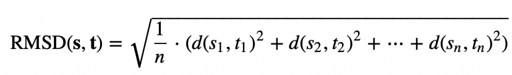
In this formula, d(si, ti) is the distance between the points si and ti.
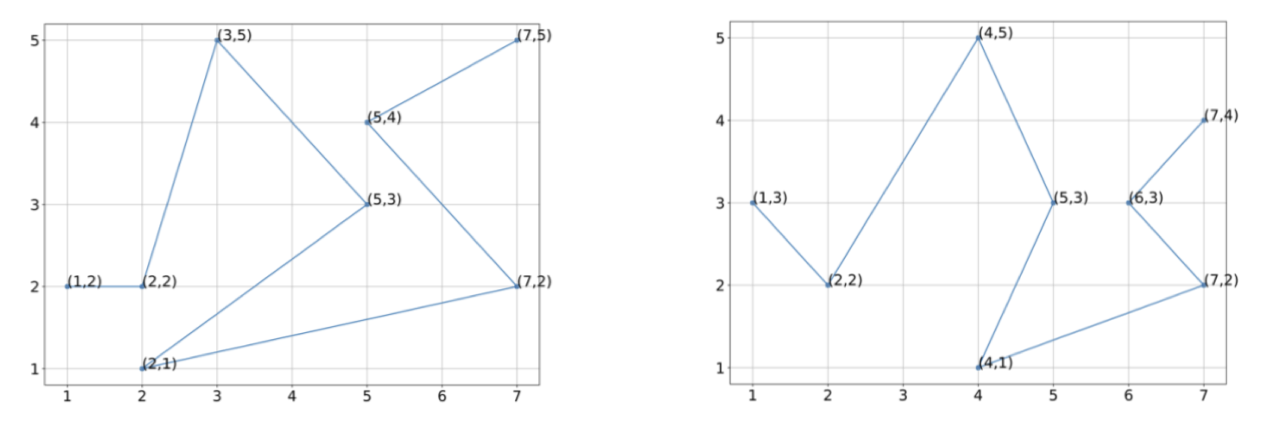
For an example two-dimensional RMSD calculation, consider the figure below, which shows two shapes with four points sampled from each. (Note: for simplicity, the shapes do not have the same center of mass.)
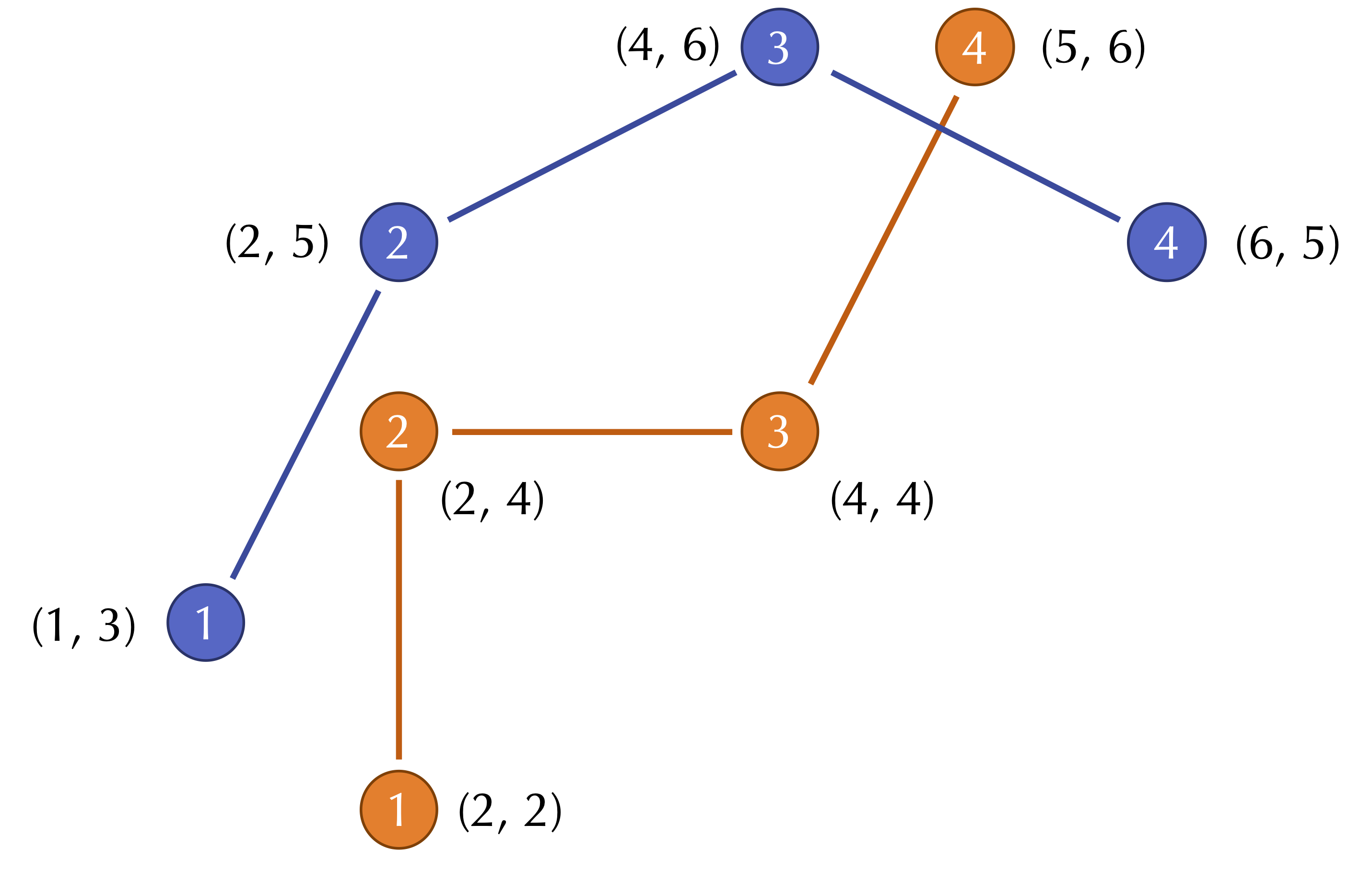
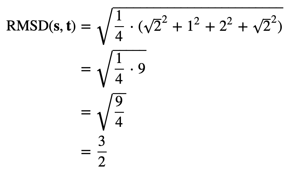
The distances between corresponding points in this figure are equal to √2, 1, 4, and √2. As a result, we compute the RMSD as
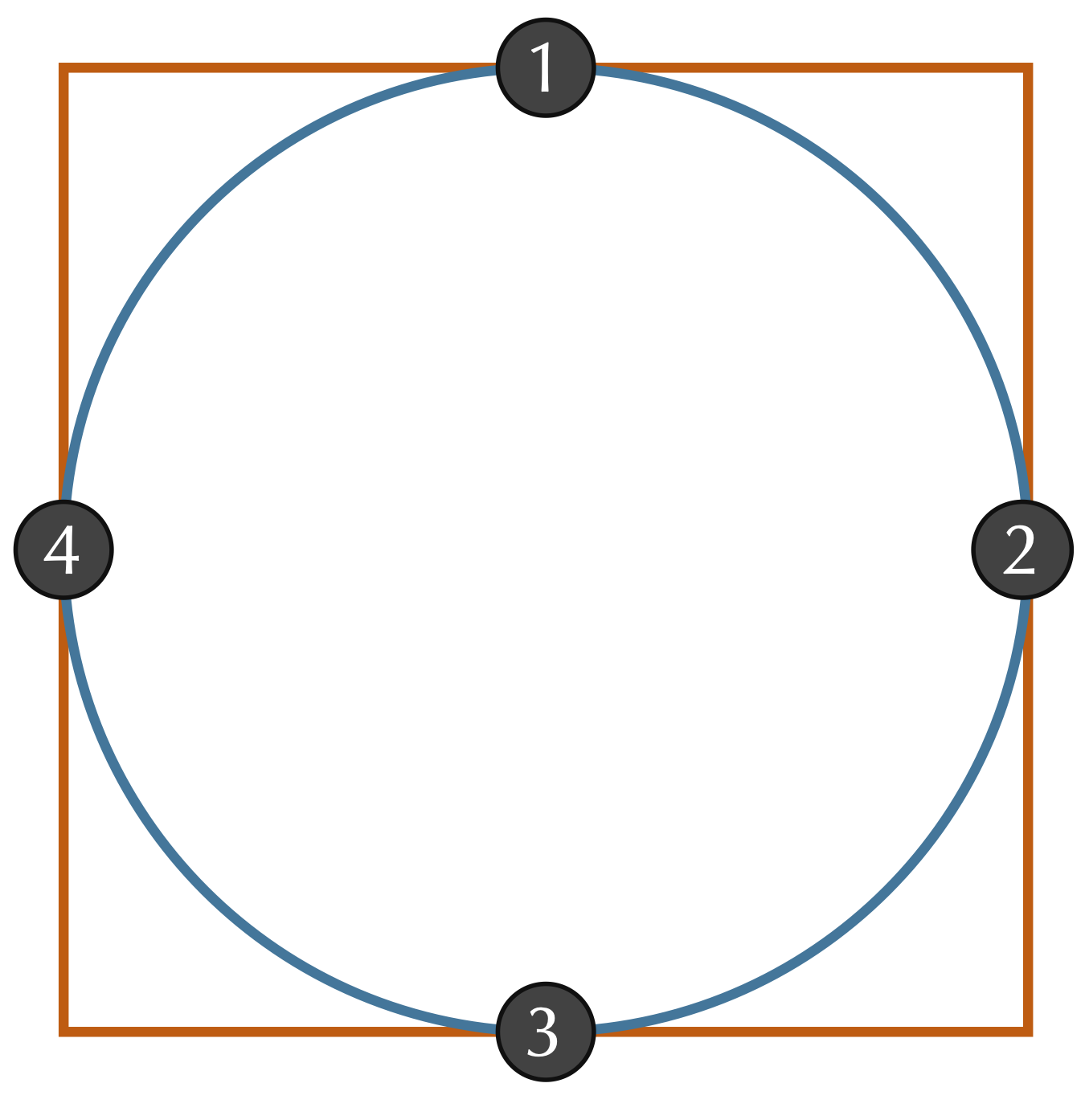
Even if we assume that two shapes have already been overlapped and rotated appropriately, we still should ensure that we sample enough points to give a good approximation of how different the shapes are. Consider a circle inscribed within a square, as shown in the figure below. If we happened to sample only the four points indicated, then we would sample the same points for each shape and conclude that the RMSD between these two shapes is equal to zero. Fortunately, this issue is easily resolved by making sure to sample enough points from the shape boundaries.
However, we have still assumed that we already rotated (and possibly flipped) S to be as “similar” to T as possible. In practice, after superimposing S and T to have the same center of mass, we would like to find the flip and/or rotation of S that minimizes the RMSD between our vectorizations of S and T over all possible ways of flipping and rotating S. It is this minimum RMSD that we define as d(S, T).
The best way of rotating and flipping S so as to minimize the RMSD between the resulting vectors s and t can be found with a method called the Kabsch algorithm. Explaining this algorithm requires some advanced linear algebra and is beyond the scope of our work but is described here.
Exercise 4: Using the vectorization of the figures indicated below, estimate the center of mass of these two protein structures.
Exercise 5: Without rotating these structures, align the two structures below so that they have the same center of mass, and determine the RMSD between the two structures for the vectorizations shown.
Comparing our structure against an experimentally verified structure
We will now use the Kabsch algorithm to compare our models against the verified structure of SARS-CoV-2. Our featured software resource is ProDy, an open-source Python package that allows users to perform protein structural dynamics analysis. Its flexibility allows users to select specific parts or atoms of the structure for conducting normal mode analysis and structure comparison.
To get started, make sure that you have the following software resources installed in order to use Jupyter Notebook. You can also access Jupyter Notebook by using Anaconda Individual Edition (we suggest downloading the graphical installer).
Next, create a directory somewhere on your computer, and move the five .pdb files that you obtained from running SWISS-MODEL to this directory. Name these files swiss_model_1.pdb, swiss_model_2.pdb, etc.
You can find a completed version of the notebook here. You may also like to follow along below as we go through this notebook.
Start Jupyter notebook by either opening Anaconda or typing jupyter notebook into a command line terminal.
Before you run the Jupyter notebook file provided, we will explain each of the components of this file. First, we have
from prody import *which imports the Prody package and can use all functions from this package.
The first built-in ProDy function that we will use, called parsePDB, parses a protein structure in .pdb format. Let’s parse in one of our models we obtained from homology modeling of the SARS-CoV-2 Spike protein, swiss_model_1.pdb.
In[#]: struct1 = parsePDB('swiss_model_1.pdb')To compare our model against the determined protein structure of the SARS-CoV-2 Spike protein, we will parse the protein with PDB ID 6vxx.
In[#]: struct2 = parsePDB('6vxx')Because the .pdb extension is missing, this command will prompt the console to search for 6vxx, the SARS-CoV-2 Spike protein, from the PDB and download the .pdb file into the current directory. It will then save the structure as the variable struct2.
With the protein structures parsed, we can now match chains. To do so, we use a built-in function matchChains with a sequence identity threshold of 75% and an overlap threshold of 80% is specified (the default is 90% for both parameters). The following function call stores the result in a 2D array called matches. In this array, matches[i] denotes the i-th match found between two chains that are stored as matches[i][0] and matches[i][1].
matches = matchChains(struct1,struct2,seqid=75,overlap=80)Let’s print out the information stored in matches. To do this, we first declare a function printMatch, which will print the sequence identity/overlap and RMSD of two polypeptide chains. Then, we have the code that calls this function for each of the rows in matches.
for match in matches:
    printMatch(match)
You can run the notebook by clicking on a block of code and clicking “run”. Do this for every block of code starting at the beginning up to the preceding code. You will see that matches[0] is Chain A from swiss_model_1 as well as Chain A from 6vxx, matches[1] is Chain A from swiss_model_1 against Chain B from 6vxx, matches[2] is Chain A from swiss_model_1 against Chain C from 6vxx, and then matches[3] starts over with Chain B from swiss_model_1 against Chain A from 6vxx.
Exercise 6: When you ran
matchChains, you most likely have in the output that the function failed to match chains initially and only succeeded when it used local sequence alignment. Why do you think this was the case? (Hint: notice the lengths of the chains.)
We want to match Chain A against Chain A (matches[0]), Chain B against Chain B (matches[4]), and Chain C against Chain C (matches[8]). That having been said, SARS-CoV-2 is a homotrimer, with all three chains very similar in structure, and the analysis below will hold up if we use another element of matches.
First, we will calculate the RMSD of Chain A from both proteins. This is satisfied by the following lines.
first_ca = matches[0][0]
second_ca = matches[0][1]
calcRMSD(first_ca, second_ca)
Run these lines. You will see that the RMSD of the two chains is very high. This is because we have not yet applied the Kabsch algorithm to ensure that the structures are correctly aligned. This alignment is provided by the calcTransformation.apply() function, which we now apply before recomputing RMSD.
calcTransformation(first_ca, second_ca).apply(first_ca);
calcRMSD(first_ca,second_ca)
Now, run this code, which should give you a more reasonable value of RMSD.
Finally, we will combine all three chains of both our predicted structure and the verified structure, and then we will apply the Kabsch algorithm and as well as calculate the RMSD of the resulting protein.
first_ca = matches[0][0] + matches[4][0] + matches[8][0]
second_ca = matches [0][1] + matches[4][1] + matches[8][1]
calcTransformation(first_ca, second_ca).apply(first_ca);
calcRMSD(first_ca, second_ca)
Run this code, and you have completed the notebook for this model.
Exercise 7: Provide a screenshot showing your finishing this part of the code to obtain an RMSD value between
swiss_model_1.pdband6vxx.pdb. Then, re-run the entire code block-by-block forswiss_model_2.pdb, and then re-run the code forswiss_model_3.pdb. Provide two more screenshots showing that you have found the RMSD values between the entire proteins of these two models and the experimentally validated SARS-CoV-2 spike protein.
Exercise 8: Change your Jupyter notebook so that you compare the experimentally validated structure of SARS-CoV-2 (6vxx) against the experimentally validated structure of SARS-CoV (6crx). What RMSD do you find? Would you say that SWISS-MODEL did a good enough job at predicting the structure of the SARS-CoV-2 protein? Explain your answer.
Comparing the SARS-CoV and SARS-CoV-2 spike protein structures locally
At the end of the last section, we compared the validated SARS-CoV and SARS-CoV-2 spike proteins. However, having just a single RMSD value does not greatly help us understand what the individual changes have been that have differentiated the SARS-CoV-2 spike protein. That is, we need to move toward comparing two structures locally.
Recall the following definition of RMSD for two protein structures s and t, in which each structure is represented by the positions of its n alpha carbons (s1, …, sn) and (t1, …, tn).

If two similar protein structures differ in a few locations, then the corresponding alpha carbon distances d(si, ti) will likely be higher at these locations. However, one of the weaknesses of RMSD is that a change to a single bond angle at the i-th position may cause d(sj, tj) to be nonzero when j > i, even though the structure of the protein downstream of this bond angle has not changed. For example, consider the following figure of two protein structures that are identical except for a single bond angle. All of the alpha carbon distances d(si, ti) for i at least equal to 4 will be thrown off by this changed angle.
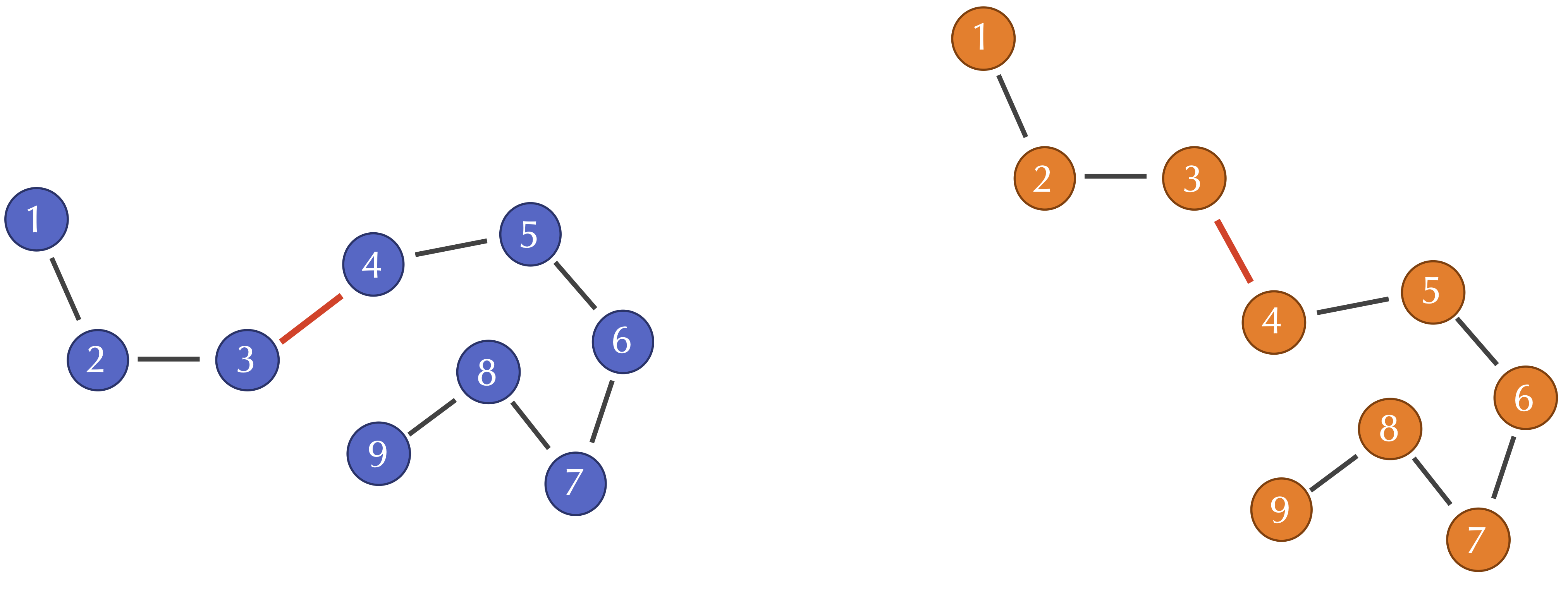
However, note that when i and j are both at least equal to 4, the distance d(si, sj) between the i-th and j-th alpha carbons in S will still be similar to the distance d(ti, tj) between the same alpha carbons in T. This observation leads us to a more robust approach for measuring differences in two protein structures, which compares all pairwise intraprotein distances d(si, sj) in one protein structure against the corresponding distances d(ti, tj) in the other structure.
To help us visualize all these pairwise distances, we will introduce the contact map of a protein structure s, which is a binary matrix indicating whether two alpha carbons are near each other in s. After setting a threshold distance, we set M(i, j) = 1 if the distance d(si, sj) is less than the threshold, and we set M(i, j) = 0 if d(si, sj) is greater than or equal to the threshold.
The figure below shows the contact maps for the SARS-CoV-2 and SARS-CoV spike proteins (both full proteins and single chains) with a threshold distance of twenty angstroms. In this map, we color contact map values black if they are equal to 1 (close amino acid pairs) and white if they are equal to 0 (distant amino acid pairs).
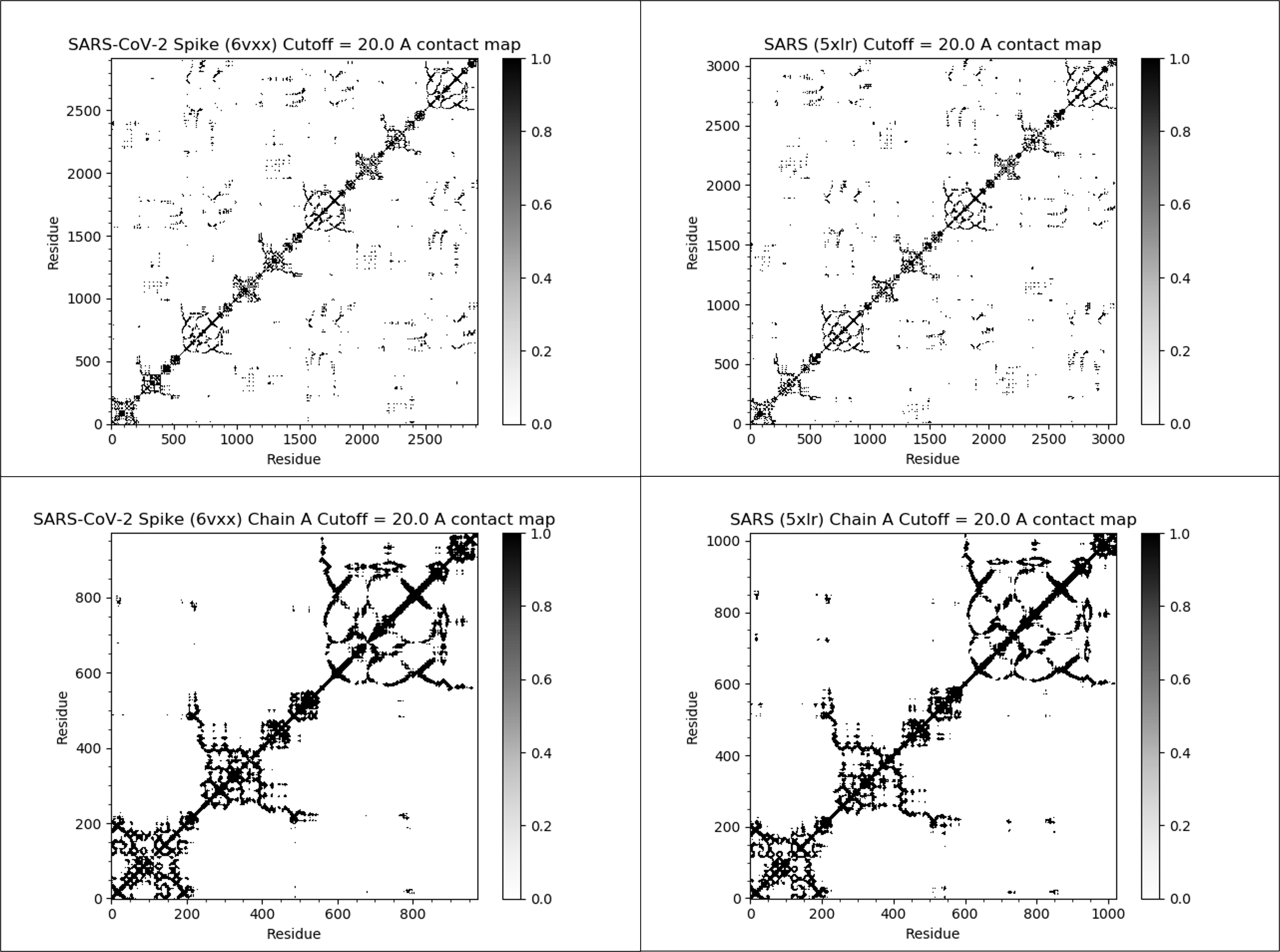
We observe two facts about these contact maps. First, many black values cluster around the main diagonal of the matrix, since amino acids that are nearby in the protein sequence will remain near each other in the 3-D structure. Second, the contact maps for the two proteins are very similar, reinforcing that the two proteins have similar structures.
We obtain some insight into how two proteins differ structurally at the i-th amino acid if we examine the values in the i-th row of the proteins’ contact maps; that is, if we compare all of the d(si, sj) values to all of the d(ti, tj) values. In practice, researchers combine all of this information into a single metric called Q per residue (Qres) measuring the similarity of two structures at the i-th amino acid. The formal definition of Qres for two structures s and t having N amino acids is
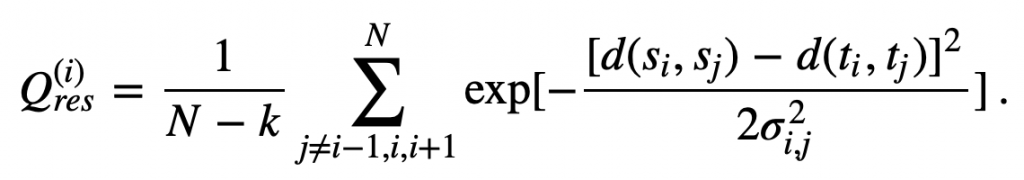
In this equation, exp(x) denotes ex. This equation also includes the following parameters.
- k is equal to 2 at either the start or the end of the protein (i.e., iis equal to 1 or N), and k is equal to 3 otherwise.
- The variance term σ2ij is equal to |i−j|0.15, which corresponds to the sequence separation between the i-th and j-th alpha carbons.
If two proteins are very similar at the i-th alpha carbon, then for every j, the difference d(si, sj) – d(ti, tj) will be close to zero, meaning that each term inside the summation in the Qres equation will be close to 1. The sum will be equal to approximately N – k, and so Qres will be close to 1. As two proteins become more different at the i-th alpha carbon, then the term inside the summation will head toward zero, and so will the value of Qres.
Qres is therefore a metric of similarity ranging between 0 and 1. Low scores indicate low similarity between two proteins at the i-th position, and higher scores indicate high similarity at this position.
Exercise 9: Consider the following figures reproduced from above. If the first sampled point in the two figures are, respectively, (1,2) and (1,3), compute the Qres of the fourth sampled point.
We now will compute Qres for the SARS-CoV and SARS-CoV-2 spike proteins, limiting our attention to a highly variable subregion of these proteins called the receptor binding domain (RBD). We will use the VMD plugin Multiseq, a bioinformatics analysis environment, to align the SARS-CoV-2 RBD and SARS RBD having the PDB entries 6vw1 and 2ajf, respectively. After calculating Qres at every position, we will identify where the two RBD regions differ and visualize these regions within the larger protein structures.
It is important to note that the experimentally verified SARS-CoV-2 structure is a chimeric protein formed of the SARS-CoV RBD in which the RBM has the sequence from SARS-CoV-2. A chimeric RBD was used for complex technical reasons to ensure that the crystallization process during X-ray crystallography could be borrowed from that used for SARS-CoV.
Multiseq aligns two protein structures using a tool called Structural Alignment of Multiple Proteins (STAMP). Much like the Kabsch algorithm discussed in class, STAMP minimizes the distance between alpha carbons of the aligned residues for each protein or molecule by applying rotations and translations. If the structures do not have common structures, then STAMP will fail. If you are interested in more details on the algorithm used by STAMP, click here.
First, download VMD. In what follows, the program may prompt you to download additional protein database information, which you should accept.
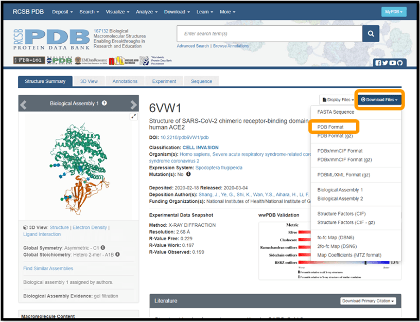
We will need to download the .pdb files for 6vw1 and 2ajf. Visit the 6vw1 and 2ajf PDB pages. For each protein, click on Download Files and select PDB Format. The following figure shows this for 6vw1.
Next, launch VMD, which will open three windows. We will not use VMD.exe, the console window, in this tutorial. We will load molecules and change visualizations in VMD Main, and we will use OpenGL Display to display our visualizations.
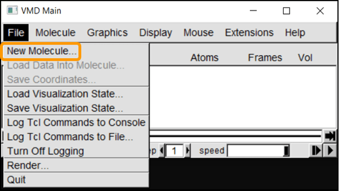
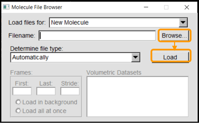
We will first load the SARS-CoV-2 RBD (6vw1) into VMD. In VMD Main, go to File > New Molecule. Click on Browse, select your downloaded file (6vw1.pdb) and click Load.
The molecule should now be listed in VMD Main, with its visualization in OpenGL Display.
In the OpenGL Display window, you can click and drag the molecule to change its orientation. Pressing ‘r’ on your keyboard allows you to rotate the molecule, pressing ‘t’ allows you to translate the molecule, and pressing ‘s’ allows you to enlarge or shrink the molecule (or you can use your mouse’s scroll wheel). Note that left click and right click have different actions.
We now will need to load the SARS-CoV RBD (2ajf). Repeat the above steps for 2ajf.pdb.
After both molecules are loaded into VMD, start Multiseq by clicking on Extensions > Analysis > Multiseq.
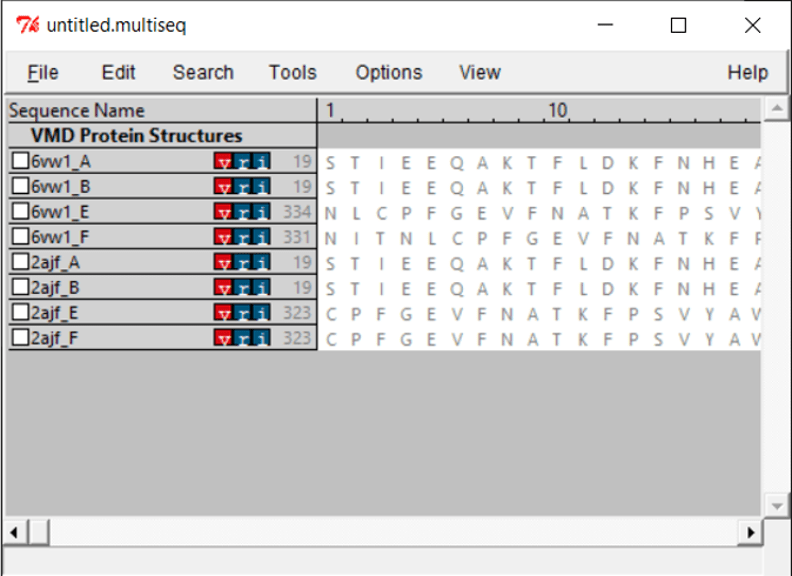
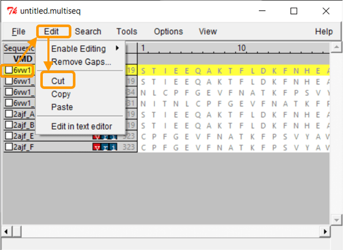
You will see all the chains listed out per file. Both .pdb files contain two biological assemblies of the structure. The first is made up of Chain A (ACE2) and Chain E (RBD), and the second is made up of Chain B (ACE2) and Chain F (RBD). Because Chain A is identical to Chain B, and Chain E is identical to Chain F, we only need to work with one assembly. (We will use the second assembly.)
Because we only want to compare the RBD, we will only keep chain F of each structure. To remove the other chains, select the chain and click Edit > Cut. You can remove the nucleic structures as well.
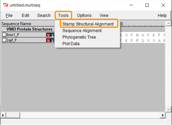
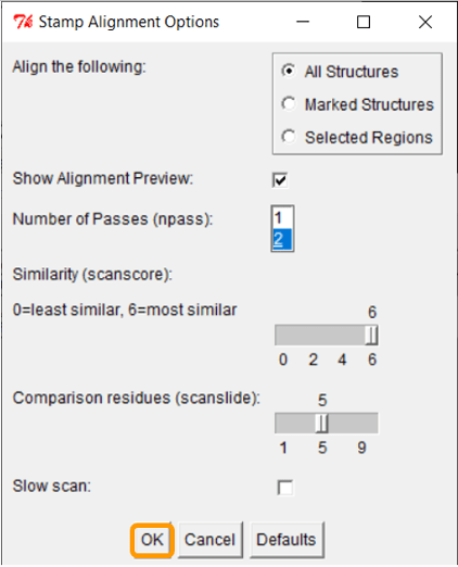
The protein structures are visible, but we need to overlap them in order to compare them visually. Click Tools > Stamp Structural Alignment, and a new window will open up.
Keep all the default settings and click OK; once you have done so, the RBD regions will have been aligned into a single structure.
Now that we have aligned the two RBD regions, we would like to compare their Qres values over the entire RBD. To see a coloring of the protein alignment based on Qres, click View > Coloring > Qres.
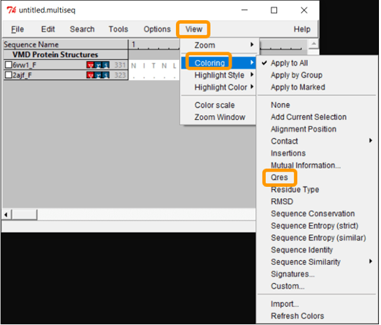
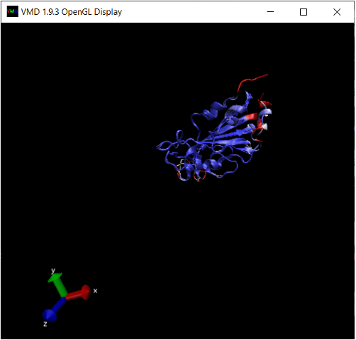
Scroll across the sequence alignment (in the untitled.multiseq window) to see how Qres changes over positions. Blue indicates a high value of Qres, meaning that the protein structures are similar at this position; red indicates low Qres and dissimilar protein structures.
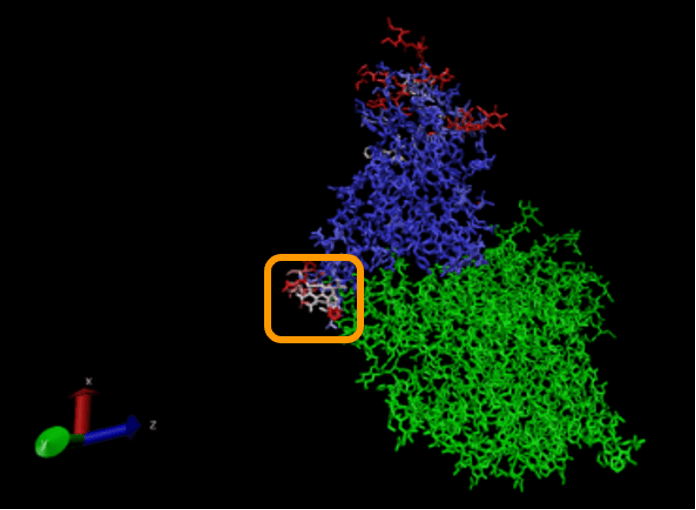
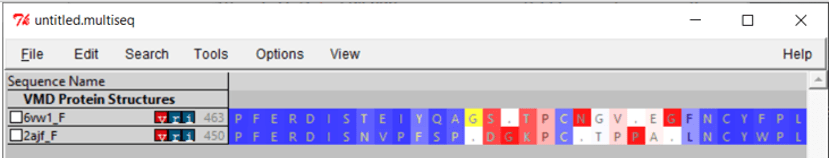
If we zoom in on the region around position 150 of the alignment, then we can see a 13-column region of the alignment within the RBD region for which Qres values are significantly lower than they are elsewhere. This region, which is shown in the figure below, corresponds to positions 476 to 486 in the SARS-CoV-2 spike protein and positions 463 to 472 in the SARS-CoV genome.
The OpenGL Display window will now color the superimposed structures according to the value of Qres. We are interested in regions of the alignment having low Qres, which correspond to locations in which the coronavirus RBDs differ structurally. Note that these regions occur on the boundaries of the RBD’s structure, where bonding is more likely to occur.
Exercise 10: There is another region in the interior of the RBD structural alignment that shows significant differences between the two protein structures. Where is it?
We won’t ask you to do this, but we can color the alignment of the proteins complexed with ACE2 according to Qres, which produces the figure below. (The ACE2 enzyme is shown in green.) The low-Qres region of the RBM alignment that we highlighted in the above figure is outlined in the figure below.
Quantifying the strength of protein binding
We found regions of local structural differences between the SARS-CoV and SARS-CoV-2 spike proteins, but so what? We know that sequence differences at the level of DNA can wind up not influencing the amino acid sequence, and in the same spirit, we should not immediately conclude that a structural change in a protein will affect its function. How, then, can we quantify the affect of this structural change?
Earlier, we searched for the tertiary structure that best “explains” a protein’s primary structure by looking for the structure with the lowest potential energy (i.e., the one that is the most chemically stable). In part, this means that we were looking for the structure that incorporates many attractive bonds present and few repulsive bonds.
To quantify whether two molecules bond well, we will borrow this idea and compute the potential energy of the complex formed by the two molecules. If two molecules bond together tightly, then the complex will have a very low potential energy. In turn, if we compare the SARS-CoV-2 RBD-ACE2 complex against the SARS-CoV RBD-ACE2 complex, and we find that the potential energy of the former is significantly smaller, then we can conclude that it is more stable and therefore bonded more tightly. This result would provide strong evidence for increased infectiousness of SARS-CoV-2.
We will compute the energy of the bound spike protein-ACE2 complex for the two viruses and see how the three regions we identified in the previous lesson contribute to the total energy of the complex. To do so, we will employ NAMD, a program that was designed for high-performance large system simulations of biological molecules and is most commonly used with VMD via a plugin called NAMD Energy. This plugin will allow us to isolate our specific region of interest to evaluate how much this local region contributes to the overall energy of the complex.
We will show how to use NAMD Energy to calculate the interaction energy for a bound complex, as well as to determine how much a given region of this complex contributes to the overall potential energy. We will use the chimeric SARS-CoV-2 RBD-ACE2 complex (PDB entry: 6vw1) and compute the interaction energy contributed by the site that we identified as a region of structural difference earlier.
To determine the energy contributed by a region of a complex, we will need a “force field”, an energy function with a collection of parameters that determine the energy of a given structure based on the positional relationships between atoms. There are many different force fields depending on the specific type of system being studied (e.g. DNA, RNA, lipids, proteins). There are many different approaches for generating a force field; for example, Chemistry at Harvard Macromolecular Mechanics (CHARMM) offers a popular collection of force fields.
To get started, download NAMD, and remember where you place it in a directory on your computer.
NAMD needs to utilize the information in the force field to calculate the potential energy of a protein. To do this, it needs a protein structure file (PSF). A PSF, which is molecule-specific, communicates between a given force field and a given molecular system. (See https://www.ks.uiuc.edu/Training/Tutorials/namd/namd-tutorial-unix-html/node23.html for more details.) Fortunately, there are programs that can generate a PSF given a force field and a .pdb file containing a protein structure. See this NAMD tutorial if you are interested in more information.
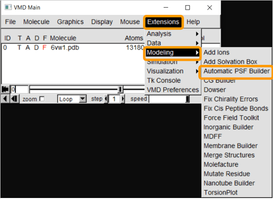
First, load 6vw1 into VMD. We then need to create a protein structure file of 6vw1 to simulate the molecule. We will be using the VMD plugin Automatic PSF Builder to create the file. From VMD Main, click Extensions > Modeling > Automatic PSF Builder.
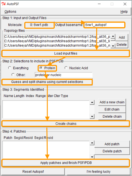
In the AutoPSF window, make sure that the selected molecule is 6vw1.pdb and that the output is 6vw1_autopsf. Click Load input files. In step 2, click Protein and then Guess and split chains using current selections. Then click Create chains and then Apply patches and finish PSF/PDB.
Notes:
- It may be the case that NAMD hangs when attempting to guess and split chains. If so, we are providing the PSF files here.
- During this process, you may see an error message stating MOLECULE DESTROYED. If you see this message, click Reset Autopsf and repeat the above steps. The selected molecule will change, so make sure that the selected molecule is 6vw1.pdb when you start over. Failed molecules remain in VMD, so deleting the failed molecule from VMD Main is recommended before each new attempt.
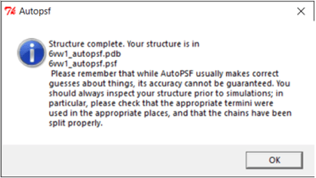
If the PSF file is successfully created, then you will see a message stating Structure complete. The VMD Main window also will have an additional line.
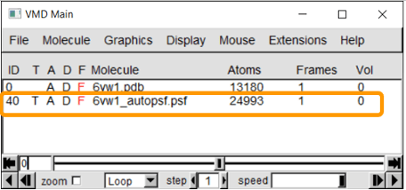
Note: If you were not able to generate the PSF file, load both the 6vw1_autopsf.psf and 6vw1_autopsf.pdb files into VMD at this point as new molecules.
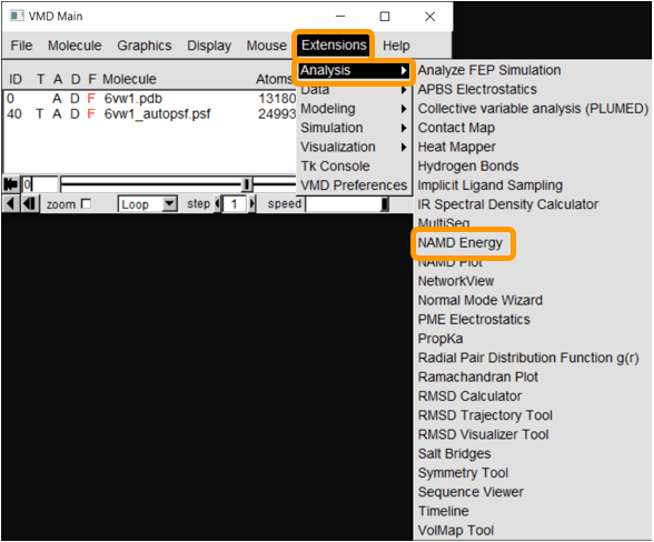
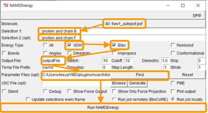
Now that we have the PSF file, we can proceed to NAMD Energy. In VMD Main, click Extensions > Analysis > NAMD Energy. The NAMDEnergy window will pop up. First, change the molecule to be the PSF file that we created.
The file 6vw1.pdb contains two biological assemblies of the complex. The first assembly contains Chain A (taken from ACE2) and chain E (taken from RBD), and the second assembly contains chain B (ACE2) and chain F (RBD). We will focus on the second assembly. Put protein and chain B and protein and chain F for Selection 1 and Selection 2, respectively.
Next, we want to calculate the main protein-protein interaction energies, divided over electrostatic and van der Waals forces. To do so, under Energy Type, check “VDW” and “Elec”.
Under Output File, enter your desired name for the results (e.g., SARS-2_RBD-ACE2_B_F). Next, we need to give NAMDEnergy the parameter file par_all36_prot.prm. This file should be found in your VMD installation at VMD > plugins > noarch > tcl > readcharmmpar1.3 > par_all36_prot.prm. (On a Mac you will need to right click on the VMD application in your Applications folder and click “Show package contents” to find these directories.) Finally, click Run NAMDEnergy. Note that you may be prompted by VMD for the location of your NAMD installation; if so, navigate to the directory where you placed NAMD and point VMD at the NAMD.exe file.
Note: If you were unable to generate the PSF file previously, then run the steps above first on 6vw1_autopsf.psf, and if this fails, try running them on 6vw1_autopsf.pdb.
The output file will be created in your current working directory (which may be your home directory if you have not set it in VMD) and can be opened with a simple text-editor. The values of your results may vary slightly upon repetitive calculations, but your results should be similar to the following. The energies here are negative because in physics, a negative value indicates an attractive force between two molecules, and a positive value indicates a repulsive force.
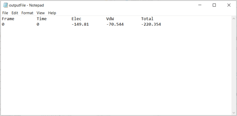
We will now compute the interaction energy contributed only by between the site of interest that we found in SARS-CoV-2 RBD loop site (residues 476 to 486) and ACE2. In the NAMDEnergy window, enter protein and chain B for Selection 1 and protein and chain F and (resid 476 to 486) for Selection 2. Keep all other settings the same.
At the close of this assignment, we ask you to compare the bonded energy between the spike protein and the human ACE2 enzyme for SARS-CoV and SARS-CoV-2. Is it the case that SARS-CoV-2 is better bound? What about in the specific regions of interest that we identified? We leave the answer to you!
Exercise 11: Compute bonded energy in this manner for chains B and F for each of SARS-CoV and SARS-CoV-2 under three conditions: globally, our region of interest (residues 476 to 486 in SARS-CoV-2; residues 463 to 472 in SARS-CoV), and the range of residues that you found in the previous exercise. Provide the results of these six analyses.
Exercise 12: Repeat the analysis from the previous exercise using chain A (ACE2) and chain E (RBD).
Exercise 13: Interpret the results of global protein analysis from the previous two exercises. How does the analysis differ depending on which chains are used? Is SARS-CoV-2 better bound to ACE2 or is SARS-CoV? (Hint: remember that negative energy means more tight bonding.)
Exercise 14: Interpret the results of local protein analysis from the previous two exercises regarding our two regions of interest. How do these two regions differ in terms of bonding energy?
Conclusion: Bamboo shoots after the rain
Despite covering a great deal of ground in this challenge, we have left just as much unstudied. For one example, the surface of viruses and host cells are “fuzzy” because they are covered by structures called glycans, or numerous monosaccharides linked together. SARS-CoV and SARS-CoV-2 have a “glycan shield”, in which glycosylation of surface antigens allows the virus to hide from antibody detection. Researchers have found that the SARS-CoV-2 spike protein is heavily glycosylated, shielding around 40% of the protein from antibody recognition.
Although the study of proteins is in some sense the first major area of biological research to become influenced by computational approaches, this area is not just still active, but booming. With the COVID-19 pandemic reiterating the importance of biomedical research, the dawn of Alphafold showing the power of supercomputing to predict structure from sequence at unprecedented accuracy, and computational modeling promising to help find the medications of the future, new companies are rising up to study proteins like bamboo shoots after the rain.
Thus concludes our discussion of protein analysis. Thank you for joining us in these challenges! If you enjoyed this effort, please consider checking out some of my other open online education projects.